Sensitivity function

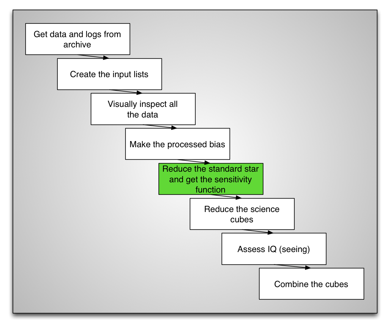
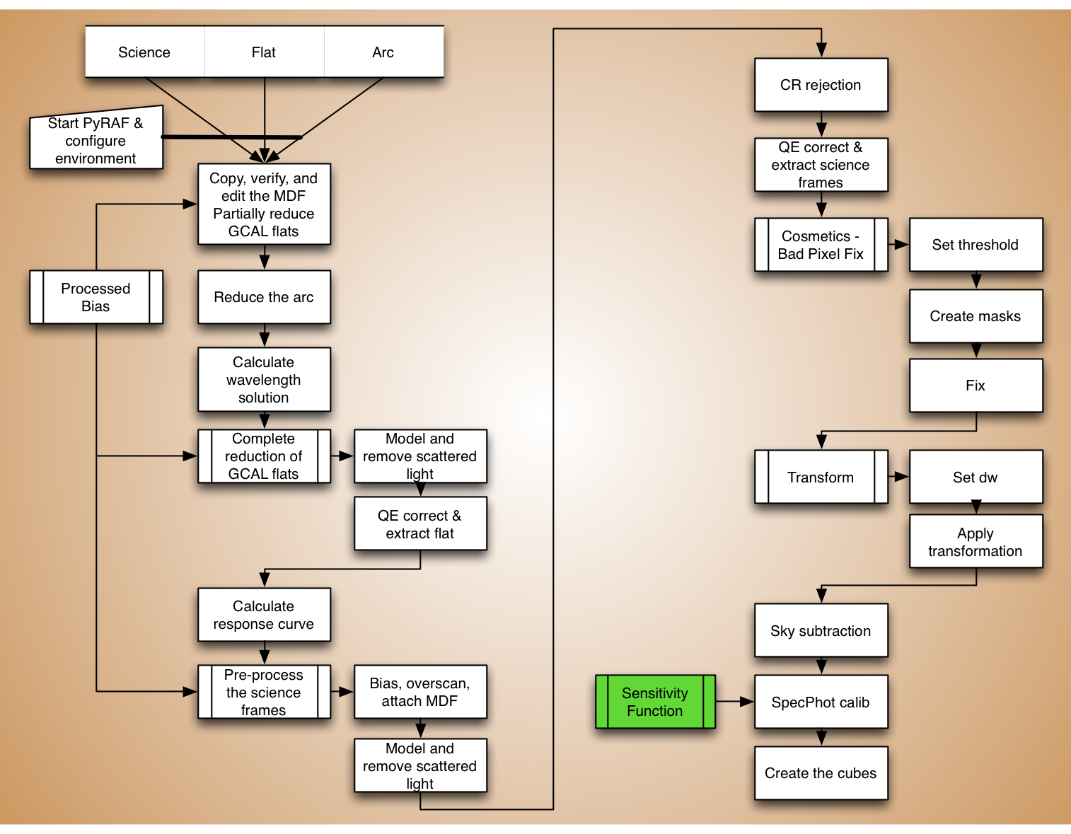
The sensitivity function is calculated from the spectrophotometric standard.

In the interest of time, we will skip the reduction of the star standard since it is essentially the same steps as for the reduction of the science, which we will cover later. We refer the reader to Appendix 1, Standard star, for an overview of the standard reduction steps.

Here we start with an already reduced standard star exposure and we proceed to demonstrate the two extra steps that will lead to the sensitivity function. Let’s copy the pre-reduced data over to redux, it is in the tutorial_data directory.

std = iraf.head('std.lis', nlines=1, Stdout=1)[0].strip()
copy('../tutorial_data/stxeqbrg'+std+'.fits', '.')

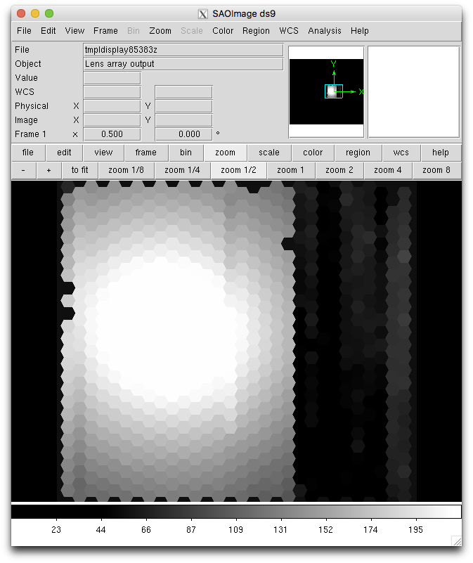
Sum the fibers

Each fiber has a spectrum of the star. In this step we sum them all to produce one single high signal-to-noise spectrum. This summing of everything also helps take away most of the differential atmospheric refraction effect by effectively using all the light in the aperture regardless of position. In the picture below, each hexagon represent a fiber, each one is a spectrum. They will all be summed together.

imdelete('astxeqbrg@std.lis')

for std in iraf.type('std.lis', Stdout=1):
    iraf.gfapsum('stxeqbrg'+std, combine='sum', fl_inter='no')

Let’s have a look a the summed spectrum.

for std in iraf.type('std.lis', Stdout=1):
    std = std.strip()
    iraf.splot('astxeqbrg'+std+'[sci,1]')

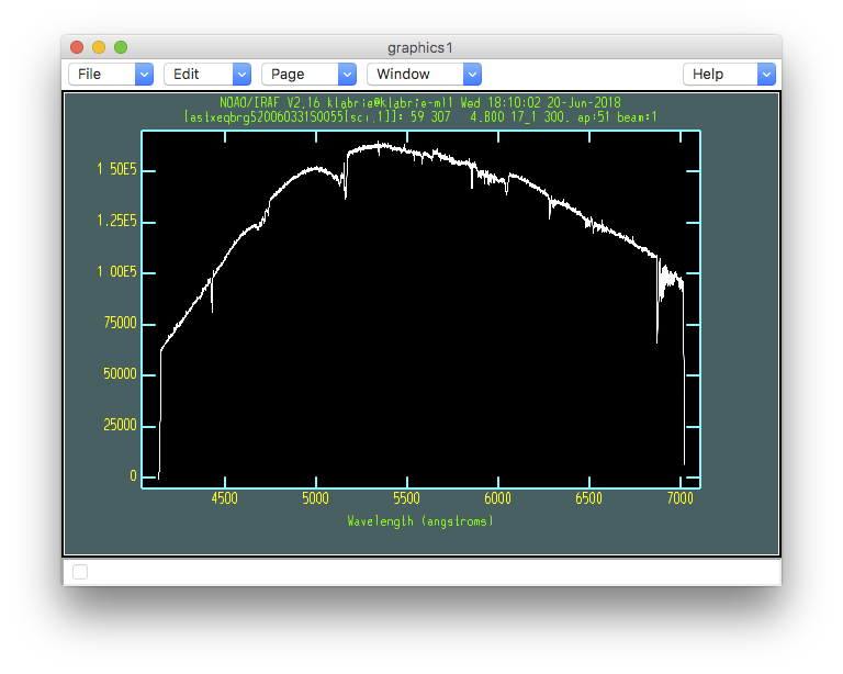
This is the shape the telescope and instrument let through. The real standard star flux does not fall off like that in the blue. That’s what the sensitivity function will correct for.

When you are ready to quit the interactive plot, press “q”.

Calculate the sensitivity function

In a very simplified picture, the sensitivity function is the difference between what was recorded and what the star spectrum really should look like. It is the shape of the spectrum that matters, not the absolute flux.

This sensitivity correction will be applied to our science observations.

Find the star

So, we need to know what the standard star spectrum looks like. IRAF provides wavelength-flux tables for a large collection of common spectrophotometric standards, for both hemispheres. Those are located in the onedstds directory. From the PyRAF session:

dir onedstds

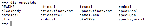
Each of these directories contains flux tables. The table for our standard star, LLT 4364, is in the subdirectory ctiocal:

dir onedstds$ctiocal

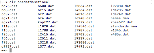
The file is named l4364.dat. It is the l4364 part that we will need to provide as starname to gsstandard below.

Set the input parameters

Now that we know in which directory our star flux table is located and what “name” IRAF uses for it, let’s define some variables we will use in the call to gsstandard.

root_name = 'ltt4364_629_20060331_'
outflux = root_name+'std'
sensfunc = root_name+'sens'

extinction = 'onedstds$ctioextinct.dat'
caldir = 'onedstds$ctiocal/'
starname = 'l4364'

input = iraf.head('std.lis', nlines=1, Stdout=1)[0].strip()

The extinction file is the CTIO site extinction file. Cerro Tololo and Cerro Pachon are right next to each other, so that extinction curve is perfectly adequate for Gemini South (Cerro Pachon). For Gemini North, one would use gmos$calib/mkoextinct.dat.

Don’t worry too much about the statement that sets the input variable. It is making use of IRAF and Python to return the first line in the file. There’s only one line in our current case, but it still need to be read and assigned to input. One could also just type the full filename in the gsstandard command, but we are trying in this tutorial to show how to minimize the modifications necessary to adapt the tutorial instructions to a different set of GMOS IFU-1 data.

Call gsstandard

We now run the task that will calculate the sensitivity function. We will run it interactively. Most of the time this is not necessary but this dataset has weak signal in the blue and a big absorption feature. It can throw the fit a bit. We can correct that interactively. Even in “normal” cases, it never hurts to run this step interactively even if just to visually verify that the fit it proposes is acceptable.

delete(outflux, verify='no')
imdelete(sensfunc, verify='no')

gsstandard('astxeqbrg'+input, outflux, sensfunc, \
           starname=starname, observatory='Gemini-South', \
           caldir=caldir, extinction=extinction, fl_inter='yes', \
           function='spline3', order=7)

- Answer 'yes' to the "Edit bandpasses" question.

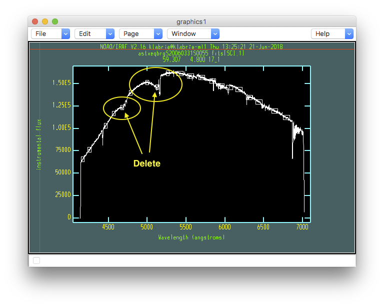
The little white boxes indicate the regions that are being used to fit the shape of the signal. As we can see in the yellow ovals, some of those regions fall on features rather than continuum.

- Point on the box to delete and type 'd'.
- To add a region (not necessary here), point and type 'a'.
- To zoom in (not necessary here), type 'w', then point to
  lower-left corner of the box you want to define and type 'e',
  then point to the upper-right corner of the zoom box and
  type 'e' again.   To zoom out, 'w', 'a'.
- When done type 'q' to move on to the next step.

- Answer 'yes' to the "Fit aperture 1 interactively?" question.

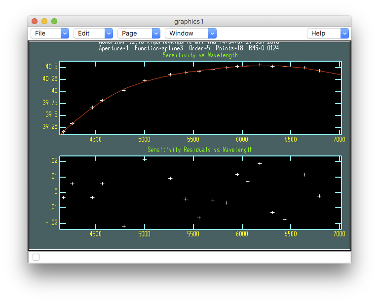
This next interactive window shows us the fitted sensitivity function.

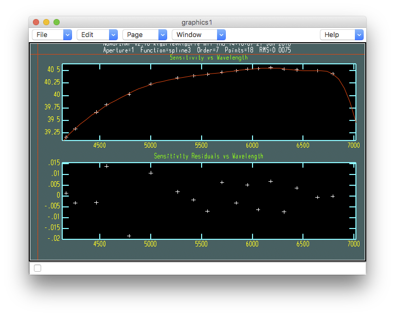
One thing at this step that you might want to change is the order of the fit. Let’s try to fix that rapid drop of the fit on the red end to get a smoother extrapolation.

- Type ":order 5", to change the order from "7" to "5".
- Then type "f" to draw the new fit, "g" to redraw with only
  the current fit.
- Type "q" when done.

Store the solution

Now that we have a carefully calculated sensitivity function, let’s move it to somewhere safe:

copy(sensfunc+'.fits', '../calibrations/')