Assessing the image quality

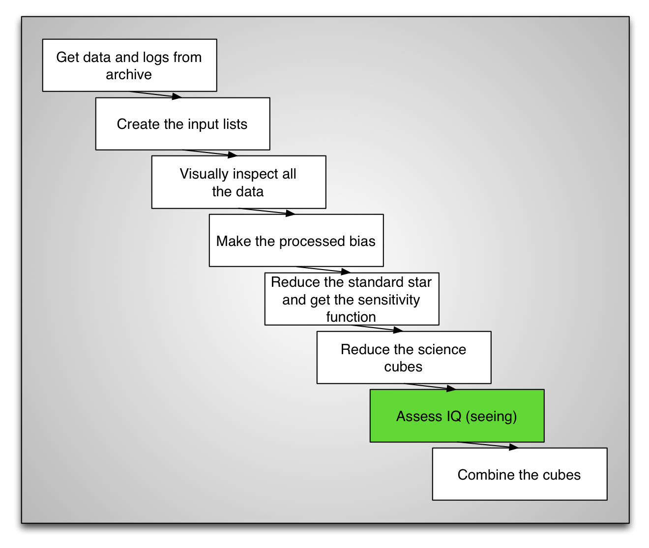
Now that we have a calibrated cube, corrected for differential atmospheric refraction (DAR) we can assess the image quality. The two things we will look at are:

1. Whether or not all the sources are in the field-of-view at all wavelengths. If the DAR is important and the source is on the edge of the field-of-view, the blue end might fall off it.
2. The seeing. Obviously, one needs a point source for that.

Inspect along wavelength axis

A good way to check whether the sources are in the FOV at all wavelength is to run a little movie that displays thick slices along the wavelength axis. To do that here, we use Python. You can copy and paste this into your PyRAF session.

The first image is a whitelight image, then the movie starts with wavelength slices 10-pixel thick. Notice at the beginning (blue) of the movie how close the top-left source is to the edge. Aperture photometry probably would not work well on that source. PSF photometry would do fine since there is enough of the source to fit a good PSF model.

import astropy.io.fits as fits
import numpy as np
import imexam
import time

display = imexam.connect(list(imexam.list_active_ds9())[0])

for sci in iraf.type('sci.lis', Stdout=1):
    sci = sci.strip()
    cube = fits.open('cstxeqxbrg'+sci+'_3D.fits')
    im = np.add.reduce(cube[1].data[500:,:,:])
    display.view(im)
    display.scale('zscale')
    time.sleep(10)
    for position in range(0, cube[1].data.shape[0], 10):
        slice = np.add.reduce(cube[1].data[position:position+10,:,:])
        display.view(slice)

Seeing

To measure the seeing we need to “collapse” the cube along the wavelength axis to create a “whitelight” image. Then we can use IRAF imexamine to fit either a Moffat or Gaussian profile to measure the Full Width at Half Maximum (FWHM) or seeing.

If you have several cubes, especially if taken on different nights, it is important to verify the seeing. It is likely that you will not want to combine good seeing cubes with bad seeing cubes. Of course that depends on your scientific objectives.

It is possible to quickly collapse the cube with the IRAF task imcombine. Below, we specify that we want to collapse the science extension, not the variance or data quality cubes, then we also specify that we want to collapse the wavelength slices starting with slice 500. The reason here is simply to ignore the very noisy blue end of the spectrum.

for sci in iraf.type('sci.lis', Stdout=1):
    sci = sci.strip()
    iraf.imdelete(sci+'_collapsed')
    iraf.imcombine('cstxeqxbrg'+sci+'_3D.fits[sci,1][*,*,500:6281]',
            sci+'_collapsed', project='yes')

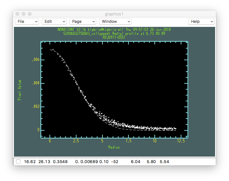
We measure the FWHM with IRAF imexamine.

for sci in iraf.type('sci.lis', Stdout=1):
    sci = sci.strip()
    iraf.imexamine(sci+'_collapsed', 1)

1. To get a radius plot (recommended), point the cursor at the center of the top-left source and type “r”.
2. If the fit looks good (dash line), you can type “a” to get the same information but with column headers so you can tell what the numbers are.
3. If the Moffat fit “does not converge”, you can switch the fit function to a gaussian profile by typing “:” then “fittype gaussian” at the prompt. To switch back to Moffat “:” followed by “fittype moffat”.

Here we find that the Gaussian fit gives us a seeing of 0.58 arcseconds (FWHM = 5.81, pixel scale = 0.1”/pixel).