QE correction and extraction of the science

We now correct the science frame for quantum efficiency effects and extract it. We use the arc for the QE correction, and we apply the response function during the extraction. Also, the extracted flat is used as a trace reference.

First let us define our variables.

flat = iraf.head('flat.lis', nlines=1, Stdout=1)[0].strip()
response = flat + '_resp'
refflat = 'eqbrg' + flat

arc = iraf.head('arc.lis', nlines=1, Stdout=1)[0].strip()

We correct for QE and complete the extraction of the science spectra.

imdelete('qxbrg@sci.lis')
imdelete('eqxbrg@sci.lis')

for sci in iraf.type('sci.lis', Stdout=1):
    sci = sci.strip()
    iraf.gqecorr('xbrg'+sci, refimage='erg'+arc, fl_correct='yes', \
            fl_vardq='yes', verbose='yes')
    iraf.gfextract('qxbrg'+sci, response=response, recenter='no', \
               trace='no', reference=refflat, weights='none', \
               fl_vardq='yes')

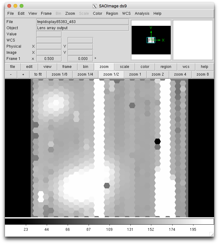
Let us have a first look at the extracted data.

for sci in iraf.type('sci.lis', Stdout=1):
    sci = sci.strip()
    iraf.gfdisplay('eqxbrg'+sci, 1, version='1')

The big white vertical lines are due to bad columns that heavily affect two fiber bundles, one target bundle, one sky bundle. It affects just a short wavelength range but gfdisplay just adds up the flux to create the image and doesn’t reject extreme values, hence the nasty artifacts.

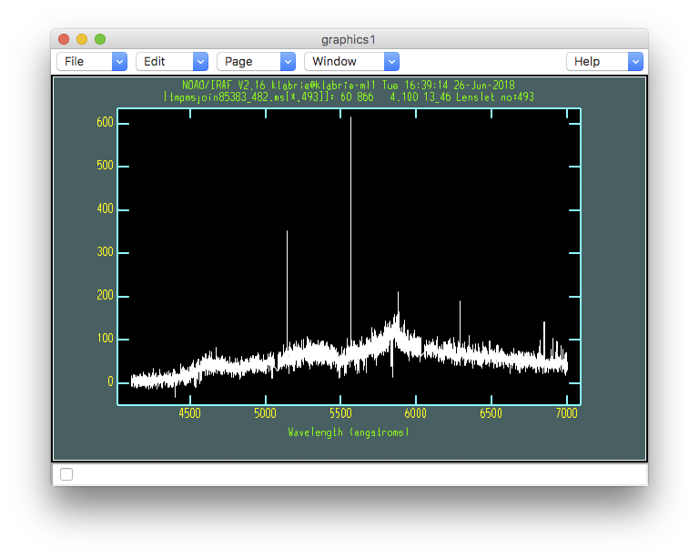
Below is the spectrum of the central fiber of the source in the top left corner. The thin spikes are sky lines. We will subtract the sky later.